The Hook Is a Property of the System

Data-Rich, Insight-Poor — CCXXIV

Explore the interactive model · View the source code on GitHub · Read the mathematical specification on GitHub · View the typeset equations

Accumulation-format reference simulations at 72 hours. The curves and molecular inventories are model outputs, not experimental measurements.

Modeling antibody–drug conjugate potency in vitro begins with a distinction that a concentration–response curve tends to conceal: the concentration added is not the exposure experienced by the intracellular payload target. Receptor engagement, internalization, sorting, processing, and productive intracellular access intervene between the administered conjugate and its biological effect (Ritchie et al.). A mechanistic model must therefore connect molecular delivery to cellular response before connecting that response to the assay signal. Fitting a potency midpoint describes the final relationship; it does not establish how that relationship was produced.

An indirect secondary-antibody–toxin assay adds another dependency. The targeting antibody and the toxin-bearing reagent are separate molecules that must assemble into a delivery-competent complex. Such systems have been used to test receptor-directed cytotoxicity, but their reagent competition is not equivalent to the behavior of a preformed ADC (Quadros et al.). The model developed here addresses this indirect format. It follows primary antibody, secondary conjugate, and receptor as distinct inventories rather than treating primary concentration as though it were already a dose of intracellular toxin.

The hook is where that distinction becomes difficult to ignore. Increasing primary antibody can reduce the eventual response even while receptor occupancy remains high. Read as a conventional potency curve, such a result could suggest a less effective targeting antibody, a resistant organoid, or a loss of activity at high dose; in the model, it can instead arise from how a finite secondary supply is partitioned among primary molecules. A monotonic fit cannot represent the declining branch, and choosing only one part of the curve changes what the reported midpoint describes. Understanding the hook is therefore necessary not merely to improve the curve, but to determine what an apparent potency difference can legitimately be attributed to.

Here, accumulation denotes an exposure format in which added reagents remain with the organoids throughout the incubation, without intervening reagent removal or medium replacement. Their free concentrations can nevertheless change as binding, transport, and uptake proceed; accumulation does not imply that every molecular inventory or signal increases continuously. The measured endpoint consequently reflects the history of a changing system. If increasing secondary removes the hook, the improved curve could reflect more productive assembly, displacement of the decline beyond the tested primary concentrations, or enough additional exposure to drive a nonlinear cell death response toward its ceiling. Establishing which of these occurred is the mechanistic problem.

The distinction is substantial even in a deliberately simplified model. At 72 hours, two simulated antibody conditions produce normalized permeability signals of 0.985 and 0.980. On an endpoint plot, they look almost interchangeable. On the model's assigned payload scale, one has delivered 9,724 productive equivalents per initial cell; the other, 3,584. Almost the same fluorescence is compatible with approximately 63% less cumulative delivery. The absolute inventories depend on that assigned scale; the relative difference survives a shared rescaling of delivery and cellular susceptibility.

The accompanying Organoid Hook Model follows this problem from reagent binding through receptor trafficking, intracellular payload, recoverable damage, and membrane-integrity fluorescence. Its 5,304 simulations use illustrative parameters and are not fitted to experimental data. Published work provides both a direct secondary-toxin cytotoxicity precedent and explicit hook observations in secondary-labeled binding and internalization assays, but these establish different parts of the argument (Quadros et al.; Shembekar et al.; Riedl et al.). None of those studies validates the complete receptor-to-CellTox sequence in tumor organoids. The model asks what follows from joining the mechanisms, and which measurements would distinguish their consequences.

Stoichiometry

In an accumulation format, free primary antibody remains available to bind the secondary conjugate in solution while receptor-bound primary recruits it at the cell surface. A homogeneous internalization assay developed by Riedl and colleagues showed a prozone effect at excess primary and discussed depletion of the secondary probe; its Fab secondary was chosen to avoid cross-linking effects (Riedl et al.). Shembekar and colleagues reported a related hook in homogeneous cell-binding fluorescence and considered increasing labeled secondary as a remedy, with a corresponding background cost (Shembekar et al.). These observations make reagent partitioning a credible mechanism, although neither study establishes how a multivalent toxin conjugate behaves in a living organoid.

A closer cytotoxicity precedent comes from Quadros and colleagues, who paired antibodies to the transcobalamin receptor CD320 with a saporin-conjugated secondary antibody in cancer-cell cultures (Quadros et al.). Excess specific primary or normal mouse IgG reduced growth inhibition, and increasing secondary from 10 to 40 nM at 2.5 nM primary produced no further increase in cell death (Quadros et al.). The experiment used an MTS endpoint in cell lines, not CellTox Green in tumor organoids, and does not establish the full dose-response behavior of the present system. It nevertheless makes two points experimentally: competition need not be restricted to receptor-binding antibody, and additional secondary need not improve the biological endpoint.

The simplest useful model allows primary antibody to bind receptor and secondary independently. It also allows a soluble primary–secondary complex to bind receptor. Excluding that last route would remove a productive path to surface assembly and could overstate sequestration; reversible complex dissociation would still return free reagents. Here, soluble complex can contribute directly to surface assembly. The hook emerges because finite secondary is distributed over an increasing primary population, while primary without secondary competes for the same receptors.

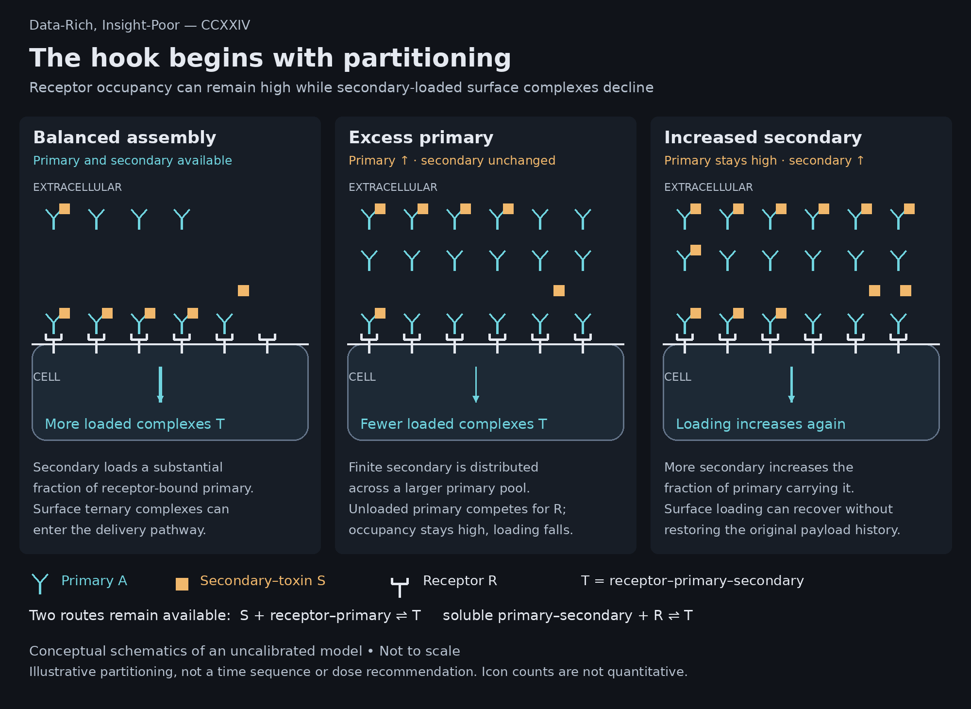
Figure 1. The assembly hook separates receptor occupancy from secondary loading. In the left panel, a substantial fraction of receptor-bound primary carries secondary conjugate. “Balanced” describes this illustrative assembly regime, not an equimolar mixture or an experimentally established optimum. In the middle panel, excess primary competes for receptors while finite secondary is distributed across a larger primary pool. In the right panel, increasing secondary at the same high primary can increase surface ternary complex. Soluble primary–secondary complex remains receptor competent in every panel, and either assembly route can contribute to T. Receptor icon number is held constant; molecular counts and arrow weights are qualitative, not the occupancies of the worked simulation. The panels depict separate conditions rather than a sequential-addition experiment. Improved loading does not establish restored cumulative payload delivery or guarantee a rescued fluorescence response. Open the full-resolution schematic.

The equilibrium limit makes that competition explicit. In a uniform compartment with effective 1:1:1 binding and negligible depletion of soluble ligands by receptor, the soluble primary–secondary complex, \(C_{\mathrm{eq}}\), determines the surface ternary complex, \(T_{\mathrm{eq}}\):

\[ \begin{aligned} C_{\mathrm{eq}}&=\frac{\Sigma-\sqrt{\Sigma^2-4A_0S_0}}{2},\\[6pt] T_{\mathrm{eq}}&=\frac{R_0\,C_{\mathrm{eq}}}{K_A+A_0}. \end{aligned} \]

Here \(A_0\) and \(S_0\) are total primary and secondary concentrations, \(R_0\) is total surface receptor concentration, and \(K_A\) and \(K_S\) are the primary–receptor and primary–secondary dissociation constants; \(\Sigma=A_0+S_0+K_S\) abbreviates their sum in the soluble binding balance. All of these variables, constants, and complex concentrations use the same concentration units. The first relationship accounts for finite secondary supply; the second accounts for competition at the receptor. At large primary excess, \(C_{\mathrm{eq}}\) approaches \(S_0\), while the competing primary concentration continues to rise. The limiting behavior is therefore particularly simple:

\[ T_{\mathrm{eq}}\sim\frac{R_0S_0}{A_0} \qquad (A_0\gg S_0,K_A,K_S). \]

Surface delivery-competent complex declines approximately in inverse proportion to primary concentration even as receptor occupancy approaches saturation. Saturating the target and supplying it with secondary conjugate have become progressively less equivalent.

This is an assembly hook without an imposed bell-shaped response function. Its maximum shifts to higher primary concentration when secondary is increased, so a titration can become monotonic over the sampled range without abolishing the high-primary decline. A general theoretical analysis of linker-mediated assembly shows that positive cooperativity can delay and mitigate a hook without eliminating it, a reminder that the independent-binding approximation will not capture every conjugate format (Dutta Roy et al.). The complete derivation gives the peak position and the conservation equations required when receptor-mediated depletion can no longer be neglected.

The opposite limit provides a useful test of the explanation. Suppose secondary is sufficiently abundant to load nearly all primary, and remains so after primary is increased tenfold. Under the same independent-binding, receptor-dilute equilibrium assumptions, the leading-order relationships become

\[ \begin{aligned} C_{\mathrm{eq}}&\approx A_0,\\[6pt] \frac{T_{\mathrm{eq}}}{R_0}&\approx\frac{A_0}{K_A+A_0} \qquad (S_0\gg A_0,K_S). \end{aligned} \]

In this approximation, increasing primary raises surface ternary assembly toward a receptor-limited plateau. With secondary fixed at 1,000 nM, primary increased from 1 to 10 nM, and dissociation constants of 1 nM for primary–receptor binding and 0.3 nM for primary–secondary binding, the receptor-dilute expression gives secondary-loaded surface fractions of approximately 0.50 and 0.91. A tenfold increase in primary therefore produces about 1.8-fold more surface ternary complex in this idealized equilibrium calculation, not tenfold more. Neither fraction measures payload delivery or killing. Receptor copies alone cannot establish the dilute limit: the cell number and accessible volume determine whether binding appreciably depletes the available primary.

The dynamic organoid model gives a different numerical answer at those same reagent concentrations. With its default geometry and 100,000 initial surface receptors per cell, surface ternary inventories at 72 hours are approximately 12,600 and 35,200 copies per initial cell, a 2.8-fold increase. Local depletion, transport, internalization, recycling, and receptor replacement are now included, and the surface inventory is no longer fixed. These review calculations are reproducible from the code but lie outside the browser atlas's precomputed secondary grid. The equilibrium example explains a limiting mechanism; it does not predict the dynamic inventory.

The qualification is in the remaining excess. A starting secondary-to-primary ratio of ten becomes one after a tenfold primary increase; a starting ratio of one thousand becomes one hundred. Equality is not itself the hook threshold. With the affinities above and secondary at 1,000 nM, the receptor-dilute assembly maximum occurs at approximately 647 nM primary, while secondary is still in about 1.55-fold nominal excess. Nominal excess does not establish that nearly every primary molecule remains secondary-loaded. The secondary-excess expression describes a limiting rise toward saturation, not a universal monotonicity rule; if receptors are already nearly saturated, increasing primary can also yield little additional assembly before any appreciable decline.

For an organoid, the relevant excess is the secondary available locally during assembly, not simply the ratio dispensed into the well. Transport and uptake can change that relationship over time. If local secondary abundance and preserved primary loading are independently established, a substantial fluorescence decline becomes evidence against simple secondary limitation as a sufficient explanation. It does not identify the alternative. Surface assembly, productive delivery, cellular susceptibility, and observation history still need to be separated; increasing assembly need not increase endpoint fluorescence if the downstream response has already reached its ceiling.

The dynamic numerical example makes the distinction between occupancy and productive assembly unusually clear. With 100,000 initial surface receptors per cell, simultaneous addition of 8.254 nM primary and 3 nM secondary yields the 0.985 fluorescence endpoint described above. At 1,000 nM primary with the same secondary concentration, modeled occupancy of the remaining surface receptor pool is approximately 99.9%, yet fluorescence falls to 0.020. Increasing secondary to 100 nM raises that signal to 0.980. Cumulative productive delivery, however, reaches only 3,584 equivalents per initial cell, compared with 9,724 in the lower-primary reference condition. Receptor occupancy was already high in the poorly killing condition; what changed was the fraction of occupied receptors carrying secondary and the exposure subsequently accumulated.

The apparent rescue therefore contains two effects: improved assembly and compression of the remaining delivery difference by the downstream response. Near its upper limit, fluorescence has little room left to report how much further one condition has progressed along the delivery pathway. A comparison based only on that endpoint would discard most of the mechanistic difference.

Receptor turnover and productive delivery

Surface abundance constrains how much antibody can bind at a given instant. Sustained delivery also depends on internalization, recycling, receptor replacement, intracellular processing, and access of the active species to its site of action, processes that need not covary with surface expression (Ritchie et al.). The model therefore gives free receptor, primary-bound receptor, and ternary complex separate internalization rates. Internalized material can recycle or enter a degradative pathway, while synthesis maintains the specified receptor abundance before treatment.

An intracellular measurement is informative only to the extent that its compartment is known. The pH-activated assay described by Riedl and colleagues detects acidified compartments but does not uniquely establish lysosomal routing; recycling further complicates interpretation of the accumulated signal (Riedl et al.). Moreover, the labeling reagent can change the route it is intended to reveal: Moody and colleagues used receptor cross-linking to redirect internalized complexes toward lysosomes (Moody et al.). Their biotin–streptavidin experiments were not secondary-toxin hook assays. They establish a consequential alternative, however: changing secondary concentration or valency may change trafficking as well as stoichiometry, an effect not generated by the fixed trafficking rates in this model.

Processing is not synonymous with productive access. In a protein-immunotoxin study, Tortorella and colleagues found more efficient formation of a cleaved active fragment along the less cytotoxic intracellular itinerary, where degradation was also faster (Tortorella et al.). In a different payload class, Tomabechi and colleagues demonstrated transport of the T-DM1 catabolite Lys-SMCC-DM1 by SLC46A3 and attenuation of T-DM1 cytotoxicity by potent transporter inhibitors (Tomabechi et al.). These findings cannot specify a common escape mechanism for different toxins. They show why internalization, processing, destructive degradation, and productive intracellular access cannot be treated as interchangeable measures of delivery.

Within each model shell, the current productive payload inventory follows

\[ \frac{dP}{dt}=\eta d\,k_{\mathrm{deg}}W_c-k_PP. \]

\(W_c\) is the endosomal ternary-complex inventory in copies per initial cell, \(k_{\mathrm{deg}}\) is its processing rate, \(d\) is the effective payload yield per secondary conjugate, and \(\eta\) is the fraction becoming productive intracellular payload. \(P\) is the current productive inventory in equivalents per initial cell, \(t\) is time in hours, and \(k_P\) is its first-order loss rate; both rate constants have units of inverse hours. The source term, \(\eta d\,k_{\mathrm{deg}}W_c\), is the delivery flux. Integrating that term gives cumulative delivery, whereas the inventory \(P\) also subtracts what has been lost. The implementation ties endosomal receptor degradation and complex processing to the same rate, with unresolved productive access represented by \(\eta\). This is a bookkeeping assumption, not a biological rule that faster receptor degradation necessarily improves toxin delivery. A system in which processing competes with toxin destruction would require those routes to be separated.

At 24 hours in the reference simulation, the population-weighted delivery flux is approximately 160 equivalents per initial cell per hour, while payload loss is 87. The current inventory is therefore increasing by about 73 equivalents per initial cell per hour and contains approximately 1,510 equivalents. The fluorescence signal is only 0.213 because damage accumulation, cell death commitment, and membrane permeabilization have their own kinetics. A payload measurement at that time and an endpoint fluorescence measurement answer different questions even when both are technically accurate.

The meaning of turnover also depends on which pool is turning over. The receptor parameter exposed in the atlas is the degradation half-time of retained endosomal receptor in the absence of recycling, rather than the measured half-life of the whole cellular receptor pool. Maintaining the same starting surface abundance while changing that rate requires a different synthesis flux. Comparisons described simply as “equal receptor expression” can therefore impose unequal replacement capacity within the model.

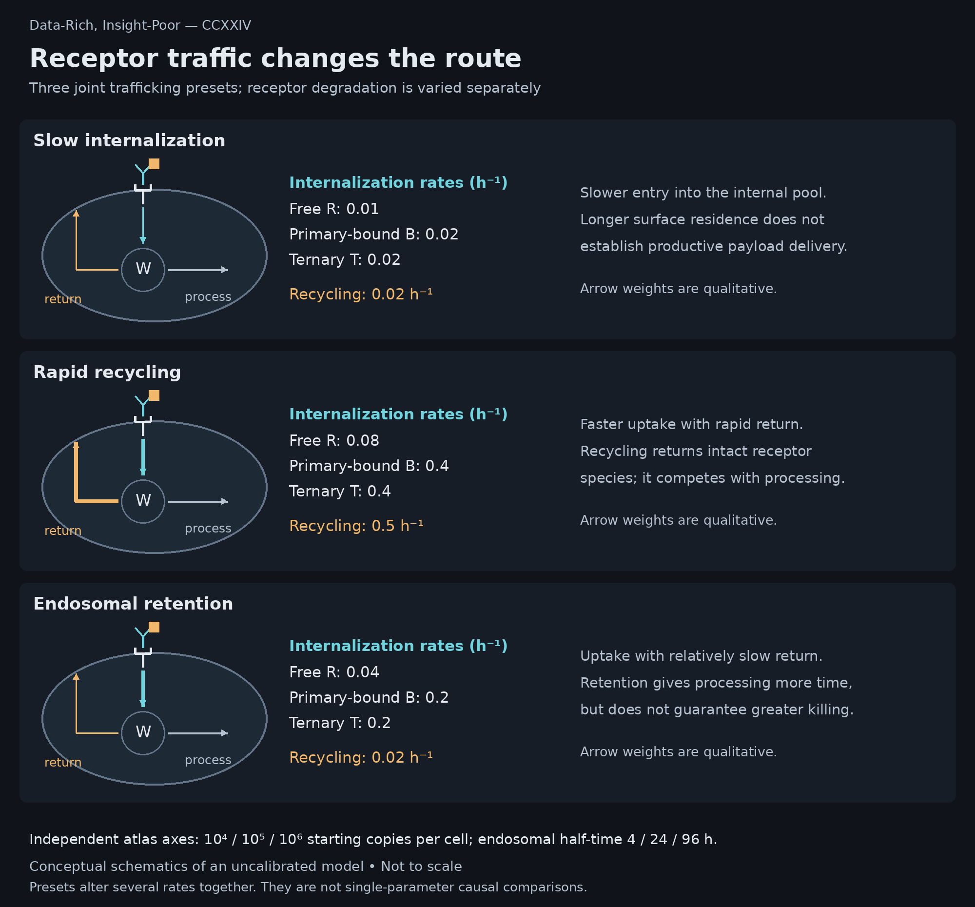
Figure 2. The receptor atlas compares three joint trafficking presets, not three isolated changes in one rate. The cellular sketches follow the internalized ternary complex; analogous internalization and recycling terms apply to free and primary-bound receptor. Initial surface copies and the conditional degradation half-time of retained endosomal receptor are independent atlas axes. Arrow weights are qualitative, and the simplified drawings omit synthesis and other unchanged terms. Open the full-resolution schematic.

Downstream recovery is represented separately as a generic reversible damage or protein-deficit state. In the reference case, sufficient damage persists to produce near-complete killing across a broad dose range. Shortening its recovery half-time from 24 to 2 hours leaves a substantial hook even at 100 nM secondary: the highest-primary fluorescence is approximately 0.226 against a sampled maximum of 0.710. Faster recovery does not create the upstream assembly deficit; it prevents that deficit from being hidden by accumulated killing. Conversely, when productive release is too poor to generate appreciable damage at any dose, a flat low curve provides no evidence that the assay has been rescued.

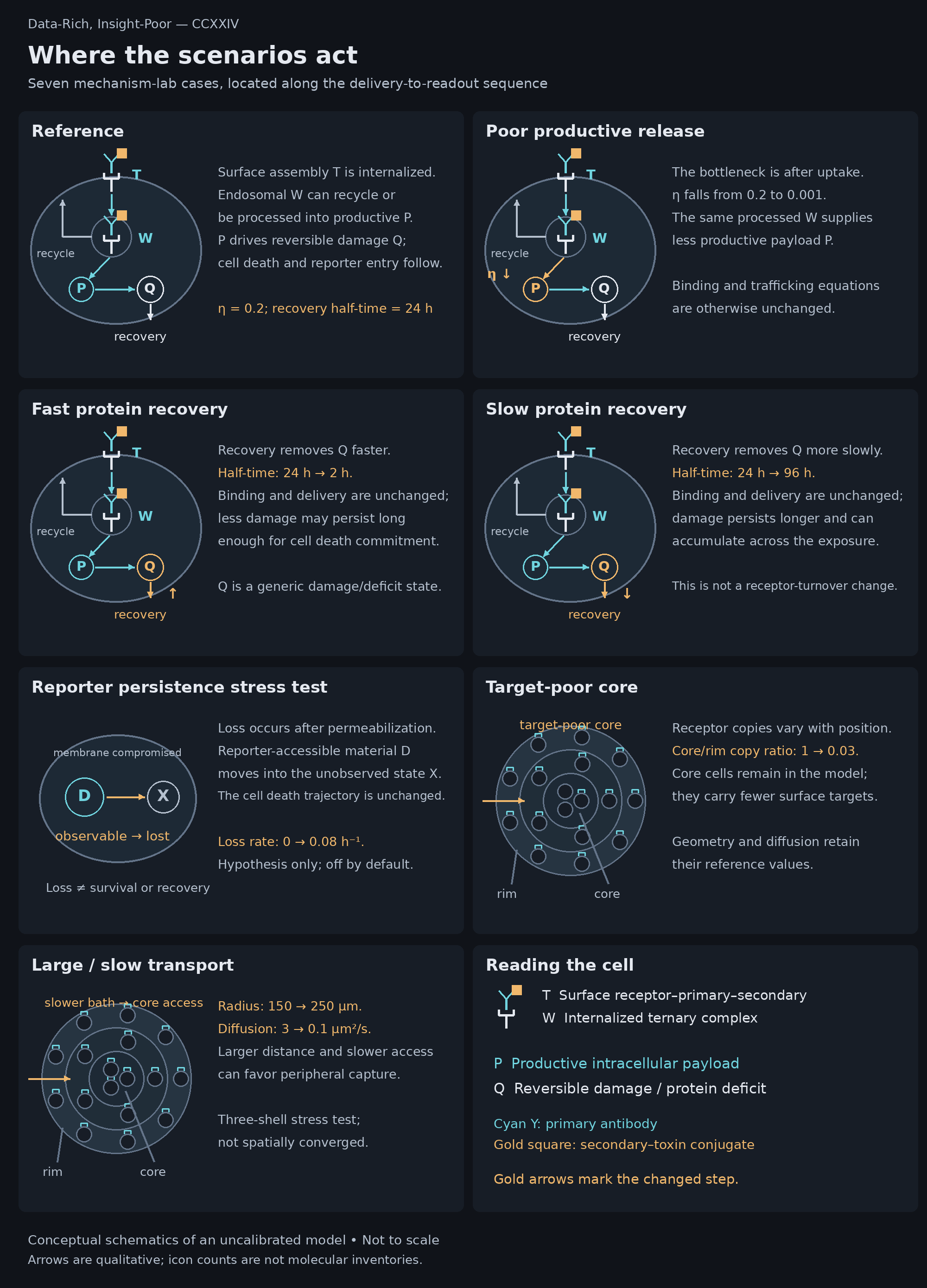
Figure 3. Each mechanism-lab scenario changes a specified part of the model relative to the reference case. T and W denote surface and internalized ternary complex; P is productive payload and Q is the generic reversible damage or protein-deficit state. The processing arrow combines several unresolved biological steps and assigns no toxin-specific route or intracellular target. Recovery is removal of Q, not export of payload from the cell. In the tissue sections, circles represent cells and cyan marks represent surface targets; their counts are illustrative, not proportional to receptor abundance, and core cells are retained in the target-poor case. Reporter loss moves already permeabilized material from an observable to an unobserved state, without restoring survival. All panels are conceptual, not calibrated predictions. Open the full-resolution schematic.

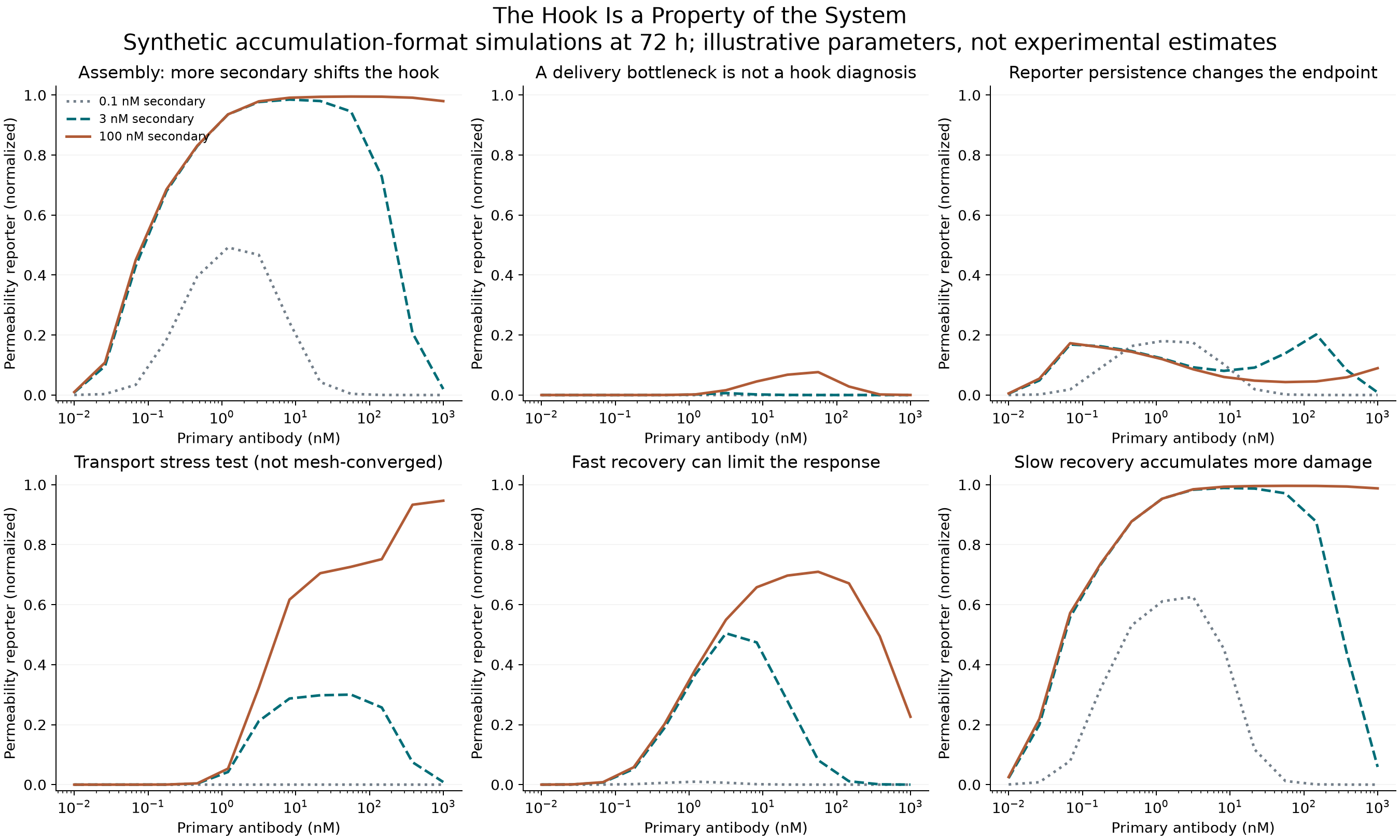
Figure 4. Accumulation-format simulations at 72 hours. The transport stress case is not spatially converged and is included to expose sensitivity to tissue geometry, not to predict penetration quantitatively.

Spatial competition

Treating receptor copy number as a whole-well scalar misses a second consequence of binding. Ackerman and colleagues experimentally examined how antigen expression and turnover affect antibody penetration into tumor spheroids, showing why a strong peripheral binding sink can restrict access to deeper tissue (Ackerman et al.). In that setting, increasing receptor abundance can favor local uptake while worsening its spatial distribution. The nominal bath concentration cannot specify both.

The converse is important. Kopp and colleagues used affinity-modulated carrier antibodies to improve the distribution of an ADC surrogate in high-expression spheroids while limiting competition in low-expression cells, then examined the strategy in vivo with ADCs (Kopp et al.). These are different reagents and experimental systems from an indirect secondary-toxin assay. Nevertheless, they provide an empirical counterweight to the assumption that receptor competition must always reduce useful delivery. Partial occupation of accessible binding sites can permit deeper penetration; its net effect depends on whether peripheral capture or insufficient cellular uptake was more limiting.

The simulator couples a finite bath to concentric tissue shells and allows free primary, free secondary, and soluble complex to diffuse separately. Binding consumes local soluble material, and intercompartmental transfer conserves its amount. Receptor expression can differ between rim and core. The three-shell representation is adequate for exploring these competing effects, but its numerical adequacy must be checked for each regime: increasing resolution to twelve shells changes reference fluorescence only slightly, whereas the large-organoid, slow-transport stress case changes substantially and nonmonotonically. That case cannot support a quantitative claim about penetration depth.

Order of addition introduces a related ambiguity in time. A delayed-secondary condition read 72 hours after the first addition has less joint exposure than a simultaneous condition read at the same clock time. The repository compares both endpoints anchored to the first addition and endpoints aligned to the availability of both reagents. Much of the apparent secondary-first delay effect in the reference simulation diminishes under the latter comparison. A claim about addition order should survive separating the order itself from the duration during which productive assembly was possible.

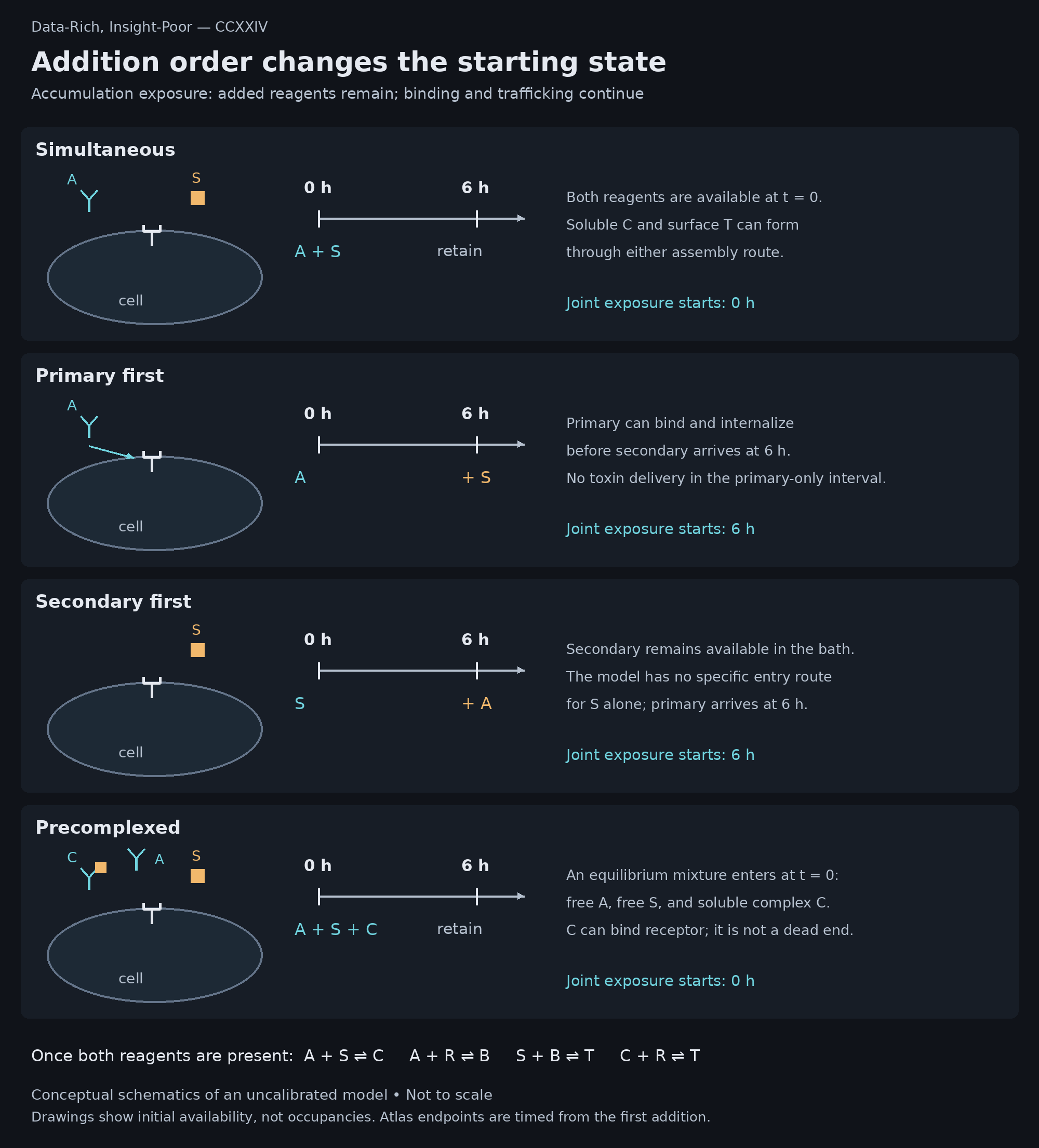
Figure 5. Addition order specifies initial availability, not an irreversible assembly route. A is primary antibody, S is secondary–toxin conjugate, C is soluble A–S complex, R is free receptor, B is receptor–primary complex, and T is receptor–primary–secondary complex. Once both reagents are present, all four reversible binding routes remain available. Delayed addition is six hours in the committed browser atlas; the Python implementation permits other delays. Precomplexing initializes an equilibrium bath mixture containing free species and complex, not complete complexation or a specified premixing duration. Reagents are retained throughout, while their free concentrations evolve. Open the full-resolution schematic.

Fluorescence and exposure history

CellTox Green reports DNA accessibility after membrane compromise, according to its technical definition, rather than receptor binding or intracellular payload (CellTox Green technical manual). Other viability methods interrogate metabolism, membrane integrity, or related cell properties through different measurement processes (Madorran et al.). Treating their outputs as interchangeable percentages assumes the biological relationships that an orthogonal assay is supposed to test.

The relevant readout evidence is not uniformly cautionary. Chiaraviglio and Kirby tested CellTox Green among impermeant DNA-binding dyes and found sustained assay separation during a three-day incubation in J774 cells (Chiaraviglio and Kirby). That supports longitudinal use under the tested conditions, without measuring a universal persistence constant or validating a matrix-embedded organoid assay. The manufacturer's protocol separately identifies compound autofluorescence, quenching, competition by DNA-intercalating compounds, and DNA fragments in extracellular matrix as possible sources of interference (CellTox Green technical manual). Those assay-specific possibilities should be investigated before a decline is assigned to an assumed loss of dead-cell reporter.

Lewis and colleagues made this issue concrete by comparing CellTox Green, LDH, MTS, and CellTiter-Glo in human intestinal organoid-derived cultures (Lewis et al.). For ritonavir in one line, the estimated CC50 was 68 μM by LDH and 73 μM by CellTox, compared with 139 μM by ATP and a value above 158 μM by MTS because the response had not crossed 50% within the tested range (Lewis et al.). The study was primarily in intestinal monolayers, with a limited 3D comparison, and explicitly left broader generalization across drugs and organoid formats unresolved (Lewis et al.). Its relevance is the experimentally demonstrated dependence of the reported response on both the culture and the assay, not a transferable correction factor for tumor organoids.

Repeated measurements also separate events that an endpoint combines. Forcina and colleagues used STACK to resolve the onset and subsequent rate of population cell death, finding substantially different kinetics among compounds with similar overall lethality (Forcina et al.). In the present model, cells accumulate damage, become committed to cell death, and then become membrane-permeable after a delay. The connection to fluorescence becomes clearer when written as an integral over that history. With no initial reporter-accessible material and a linear observation process, the normalized signal is

\[ F(t)=\sum_j\omega_j \int_0^t r_j(u)\,e^{-k_{\mathrm{loss}}(t-u)}\,du. \]

The index \(j\) identifies a tissue shell, and \(u\) is the earlier time at which cells became permeable. The entry rate \(r_j(u)\), measured as a fraction of that shell's initial cells per hour, equals \(k_{\mathrm{perm}}E_j(u)\): \(E_j\) is the fraction committed to cell death but not yet permeable, and \(k_{\mathrm{perm}}\) is the first-order permeabilization rate in inverse hours. The normalized optical weight \(\omega_j=w_jo_j/\sum_\ell w_\ell o_\ell\) combines the shell's initial-cell fraction \(w_j\) with its relative optical contribution \(o_j\); \(\ell\) runs over the same shells. Finally, \(k_{\mathrm{loss}}\) is the first-order loss rate of reportable material. Thus \(F\) is dimensionless and referenced to complete, persistent permeabilization of the initial population, rather than calibrated fluorescence units.

With \(k_{\mathrm{loss}}=0\), every past entry into the permeable state retains equal weight within its shell. Fluorescence accumulates a record of membrane compromise, even after the intracellular payload responsible for it has declined. A positive loss rate progressively discounts older events. The equation separates two histories that an endpoint otherwise conflates: when cells became permeable and how much of that event remains observable at the time of reading.

Reporter loss illustrates a mathematical possibility, not an established explanation for this CellTox assay. In an optional simulation, approximately 99% of the initial population has committed to cell death at the highest primary concentration, while normalized fluorescence is only about 9%, because reportable material has been allowed to disappear after permeabilization. Earlier killing leaves more time for that loss. The same cell death trajectory therefore produces different endpoint curves depending on whether the reporter remains observable; the simulated difference is not evidence that such loss actually occurs.

There is a relevant precedent, with an important boundary. Forcina and colleagues observed occasional declines in SYTOX Green-positive object counts, attributed most likely to marker loss from long-dead cells, and incorporated a correction into their lethal-fraction analysis (Forcina et al.). This involved a different dye and counted objects rather than whole-well fluorescence. It motivates measuring persistence in the assay of interest, but supplies neither evidence of CellTox Green decay nor a loss constant for this model. Reporter loss remains off by default. Monotonic detector saturation is a separate issue: it can conceal differences or flatten an increasing response, but cannot by itself reverse the direction of a monotonic input.

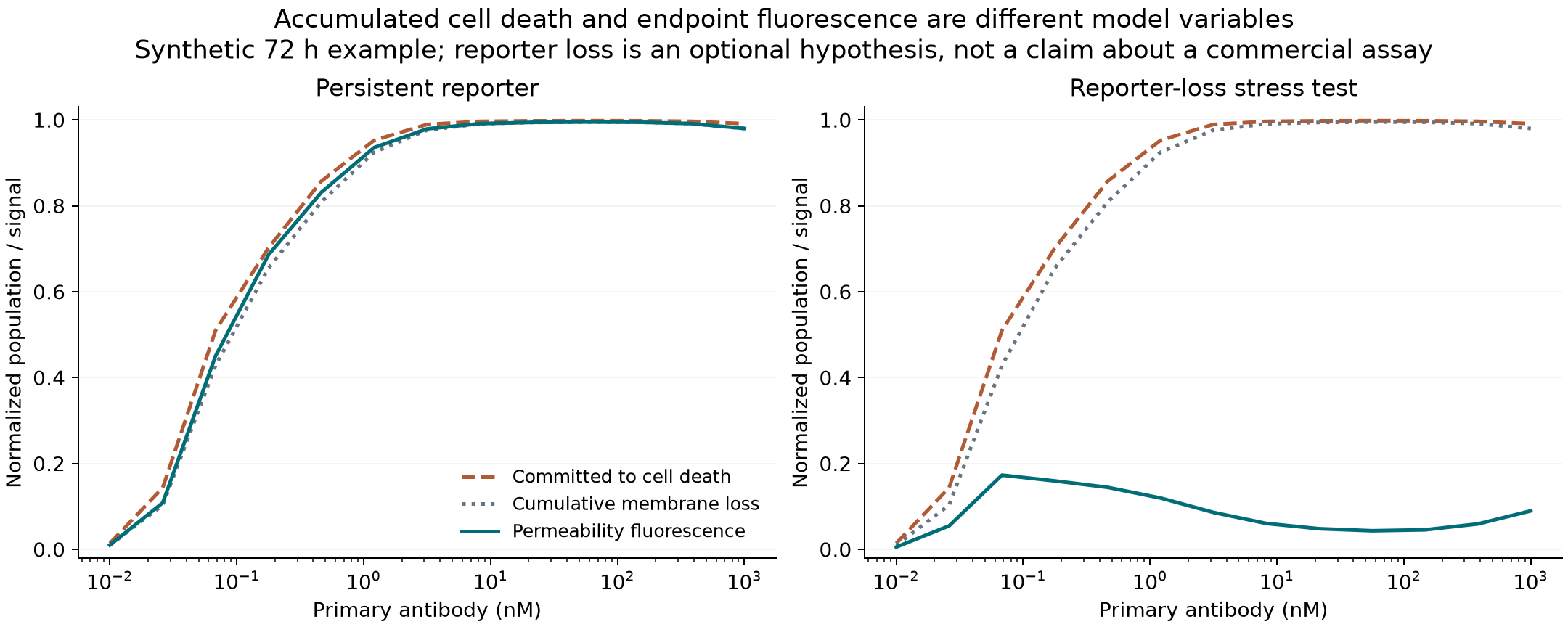
Figure 6. Cumulative cell death commitment, membrane permeabilization, and fluorescence with reporter loss disabled or enabled. The loss scenario changes the observation process without changing the underlying killing trajectory. It is an unvalidated observation-model stress test, not a measured property of CellTox Green; reporter loss is disabled in the reference model.

Extending the analysis to ATP requires more than replacing the reporter equation. Hafner and colleagues showed that conventional endpoint drug-response metrics depend on the number of divisions during an assay and introduced growth-rate inhibition metrics to address that confounding (Hafner et al.). The current simulator contains no proliferation. Its ATP-like, LDH-like, and committed-state readouts are alternative observations of a fixed initial population, not calibrated commercial assays or growth-rate-corrected sensitivity estimates.

Discriminating mechanisms

The useful next measurement depends on what the proposed explanation must account for. If secondary limitation is dominant, increasing secondary should alter surface ternary assembly as well as the final response. If assembly improves while intracellular payload remains inadequate, trafficking and productive processing become the more informative quantities. A spatial explanation requires evidence of redistribution between accessible and poorly reached cells; a bulk increase in antibody uptake is insufficient. A reporter explanation requires divergence between the independently measured biological trajectory and the material that remains observable.

A primary-by-secondary concentration matrix, paired with time-resolved assembly, delivery, and cell-state measurements, would therefore constrain more than a dense primary titration read once. Target-negative, primary-only, and secondary-only conditions are particularly consequential because nonspecific uptake and toxicity are absent from the model. A secondary-only signal cannot be accommodated honestly by adjusting receptor affinity. A matched nonbinding IgG competitor asks a different question: whether secondary can be diverted without occupying the target, as the Quadros experiment demonstrates (Quadros et al.). Its effect would not by itself establish nonspecific killing. Likewise, failure of the assembly maximum to shift as predicted, under conditions where equilibrium and negligible depletion are defensible, would challenge the independent-binding approximation before any downstream cell death parameter needed to be fitted.

Some mismatches will require a different model. Effective 1:1:1 binding omits cross-linking and avidity; there is no aggregate distribution, extracellular cleavage, bystander payload transport, growth, or changing tissue geometry. Trafficking also continues on a fixed initial-cell population after cell death commitment, which can overestimate late delivery. The reported molecular inventories are consequently per initial cell, not per surviving cell. These limitations matter especially when an endpoint approaches complete killing, precisely where continued modeled delivery becomes least biologically secure.

Calibration and prediction

The model is uncalibrated: its parameter values have not been estimated against matched experimental measurements from a defined antibody, conjugate, receptor, and organoid system. The reported hook positions, delivery inventories, and fluorescence values are therefore conditional consequences of the chosen assumptions, not quantitative predictions for a particular assay. The 5,304 simulations explore that assumed system; their number does not supply experimental support for it. The software tests address mathematical bookkeeping and numerical behavior, leaving the biological accuracy of the inputs and structure to experimental evaluation.

Calibration would begin by constraining the model with measurements that distinguish its stages: accessible receptor copies, binding and complex formation, trafficking and intracellular processing, and time-resolved cell-state and reporter responses. Independently measured quantities would set inputs or defensible bounds; the remaining parameters would be estimated jointly from complementary observations across concentrations and times, with measurement error and preparation-to-preparation variability carried into the uncertainty analysis. A fluorescence titration alone would leave important ambiguities. In this model, for example, payload yield and productive-release efficiency enter the delivery term as a product; even excellent agreement with the final curve cannot identify them separately without additional information. Where the data constrain only such a combination, that combination should be reported rather than assigning unwarranted precision to its components.

The ambiguity extends to the absolute delivery scale. Damage production depends on payload relative to its half-maximal response scale, \(P_{50}\), which is expressed in the same equivalents-per-initial-cell units as \(P\). Doubling productive-release efficiency and \(P_{50}\) together doubles productive payload while preserving that relative exposure and, consequently, the modeled fluorescence trajectory. In a numerical check, cumulative delivery at 72 hours rises from approximately 9,724 to 19,449 equivalents per initial cell while fluorescence remains 0.985; differences across the computed trajectory are below 0.000001. This is structural nonidentifiability, not merely an insufficiently dense titration. More fluorescence observations cannot distinguish parameter sets that the observation model makes equivalent. An independently constrained payload scale or cellular susceptibility is needed to break that equivalence.

The opening comparison survives this particular ambiguity: a shared rescaling multiplies both delivery inventories equally and leaves the approximately 63% reduction unchanged. That does not make the ratio identifiable from fluorescence alone, nor guarantee its stability after other biological parameters change. It makes the relative deficit robust to this specific scale symmetry within the chosen model. Converting receptor copies into concentration is a geometric accounting step; assigning productive payload equivalents and predicting instrument fluorescence require additional biological and measurement calibration.

A calibrated fit would still require validation against observations withheld from parameter estimation, preferably including independent organoid preparations and exposure conditions. The relevant test is whether the model predicts those responses, with useful uncertainty bounds, without being readjusted to each result. Persistent, structured errors would call for revisiting the model's biology, observation process, or spatial resolution before further parameter tuning. This progression could support quantitative use within a defined experimental domain; it would not establish that the inferred mechanism is unique or that the same calibration transfers to another receptor, conjugate, or assay.

The tool

The Organoid Hook Model makes the sequence examined in this article accessible in a browser, without installation. Its underlying Python implementation solves coupled differential equations for antibody binding, receptor internalization and recycling, intracellular processing, productive payload, recoverable damage, and transitions toward membrane compromise. A finite external bath exchanges material with three concentric organoid shells, allowing local receptor abundance and tissue access to influence delivery. Fluorescence and the alternative assay proxies are calculated from those evolving states through separate observation equations.

The browser offers two complementary views. The receptor atlas compares selected receptor copy numbers, trafficking behaviors, endosomal degradation half-times, addition orders, and observation times across primary and secondary concentrations. The mechanism lab examines specified changes in transport, core expression, productive release, downstream recovery, or reporter persistence. Switching the plotted quantity from fluorescence to surface complex, intracellular payload, or cumulative delivery exposes where two apparently similar response curves cease to agree. Exact values, parameter files, and chart exports make those comparisons inspectable beyond the screen.

Begin with the Start here guide, then change one assumption and ask whether fluorescence and productive delivery still tell the same story. The aim is not to predict your assay, but to examine which interpretations survive the comparison.

For a closer view, Follow one simulation traces a fixed reference system across six time points and three reagent conditions. It connects the initial receptor inventory to surface assembly, intracellular delivery, damage, cell death commitment, and fluorescence, with downloadable trajectories and a reproduction script. This walkthrough is independent of the main explorer controls; its purpose is to make the molecular accounting explicit before introducing the larger parameter space. The worked example supplies the numerical substitutions, while the mathematical specification defines the full equations, variables, units, and assumptions.

The source code on GitHub includes the Python solver, editable parameter examples, a notebook, automated tests, simulation outputs, and the public-source audit. The browser displays 5,304 precomputed simulations from that implementation; it does not solve new parameter combinations, interpolate between scenarios, or fit an experimental curve. Readers who want to change continuous parameters, exposure duration, or addition delays can run the Python package and generate new trajectories. Keeping the executable model and its assumptions available alongside the figures makes it possible to test how an interpretation depends on the choices that produced it.

The model therefore supports a narrower, more useful conclusion than “excess primary consumes the secondary.” Finite secondary can generate a genuine assembly hook even when soluble complexes remain receptor competent. Increasing secondary can move that hook, increase delivery, or conceal a remaining deficit behind a near-saturated cell death response. Published trafficking experiments make clear that a real multivalent reagent may also change the route, rather than merely the amount, of uptake (Moody et al.). Rescue of fluorescence cannot choose among these explanations.

The nearly superimposable endpoints in the opening example are therefore not evidence of equivalent delivery, and a persistent hook under verified local secondary excess is not evidence of reporter failure. Each is a constraint on an explanation, not the explanation itself. The decisive question is which measured intermediate changes when the curve changes: secondary loading, productive intracellular payload, the cellular response to that payload, or the observation of membrane compromise. A model earns its place here by making those alternatives distinguishable and its own assumptions falsifiable, not by turning an ambiguous curve into a confident diagnosis.

References

1. Quadros EV, Nakayama Y, Sequeira JM. Targeted delivery of saporin toxin by monoclonal antibody to the transcobalamin receptor, TCblR/CD320. Molecular Cancer Therapeutics. 2010;9:3033–3040. doi:10.1158/1535-7163.MCT-10-0513. Full text.

2. Riedl T, van Boxtel E, Bosch M, Parren PWHI, Gerritsen AF. High-Throughput Screening for Internalizing Antibodies by Homogeneous Fluorescence Imaging of a pH-Activated Probe. Journal of Biomolecular Screening. 2016;21:12–23. doi:10.1177/1087057115613270. Full text.

3. Shembekar N, Hu H, Eustace D, Merten CA. Single-Cell Droplet Microfluidic Screening for Antibodies Specifically Binding to Target Cells. Cell Reports. 2018;22:2206–2215. doi:10.1016/j.celrep.2018.01.071. Full text.

4. Dutta Roy R, Rosenmund C, Stefan MI. Cooperative binding mitigates the high-dose hook effect. BMC Systems Biology. 2017;11:74. doi:10.1186/s12918-017-0447-8. Full text.

5. Ritchie M, Tchistiakova L, Scott N. Implications of receptor-mediated endocytosis and intracellular trafficking dynamics in the development of antibody drug conjugates. mAbs. 2013;5:13–21. doi:10.4161/mabs.22854. Full text.

6. Tomabechi R, Kishimoto H, Sato T, Saito N, Kiyomiya K, Takada T, Higuchi K, Shirasaka Y, Inoue K. SLC46A3 is a lysosomal proton-coupled steroid conjugate and bile acid transporter involved in transport of active catabolites of T-DM1. PNAS Nexus. 2022;1:pgac063. doi:10.1093/pnasnexus/pgac063. Full text.

7. Ackerman ME, Pawlowski D, Wittrup KD. Effect of antigen turnover rate and expression level on antibody penetration into tumor spheroids. Molecular Cancer Therapeutics. 2008;7:2233–2240. doi:10.1158/1535-7163.MCT-08-0067. Full text.

8. Kopp A, Dong S, Kwon H, Wang T, Desai AA, Philippart A, Koo DJ, Linderman JJ, Tessier PM, Thurber GM. In vivo Auto-tuning of Antibody-Drug Conjugate Delivery to Maximize Efficacy using High-Avidity, Low-Affinity Antibodies. Molecular Cancer Therapeutics. 2026;25:610–621. doi:10.1158/1535-7163.MCT-25-0576. Full text.

9. Lewis MA, Patil K, Ettayebi K, Estes MK, Atmar RL, Ramani S. Divergent responses of human intestinal organoid monolayers using commercial in vitro cytotoxicity assays. PLOS ONE. 2024;19:e0304526. doi:10.1371/journal.pone.0304526. Full text.

10. Forcina GC, Conlon M, Wells A, Cao JY, Dixon SJ. Systematic Quantification of Population Cell Death Kinetics in Mammalian Cells. Cell Systems. 2017;4:600–610.e6. doi:10.1016/j.cels.2017.05.002. Full text.

11. Hafner M, Niepel M, Chung M, Sorger PK. Growth rate inhibition metrics correct for confounders in measuring sensitivity to cancer drugs. Nature Methods. 2016;13:521–527. doi:10.1038/nmeth.3853. Full text.

12. Madorran E, Ambrož M, Knez J, Sobočan M. An Overview of the Current State of Cell Viability Assessment Methods Using OECD Classification. International Journal of Molecular Sciences. 2025;26:220. doi:10.3390/ijms26010220. Published online December 30, 2024. Full text.

13. Moody PR, Sayers EJ, Magnusson JP, Alexander C, Borri P, Watson P, Jones AT. Receptor Crosslinking: A General Method to Trigger Internalization and Lysosomal Targeting of Therapeutic Receptor:Ligand Complexes. Molecular Therapy. 2015;23:1888–1898. doi:10.1038/mt.2015.178. Full text.

14. Tortorella LL, Pipalia NH, Mukherjee S, Pastan I, Fitzgerald D, Maxfield FR. Efficiency of Immunotoxin Cytotoxicity Is Modulated by the Intracellular Itinerary. PLOS ONE. 2012;7:e47320. doi:10.1371/journal.pone.0047320. Full text.

15. Chiaraviglio L, Kirby JE. Evaluation of Impermeant, DNA-Binding Dye Fluorescence as a Real-Time Readout of Eukaryotic Cell Toxicity in a High Throughput Screening Format. Assay and Drug Development Technologies. 2014;12:219–228. doi:10.1089/adt.2014.577. Full text.